Multi-Armed Bandit (MAB)

multi-armed-bandit

Multi-Armed Bandit (MAB) 이란?

Multi-Armed Bandit (MAB)은 카지노에서 보상을 극대화하기 위해 최적의 슬롯머신(“arm”)을 선택하는 문제에서 영감을 받은 적응형 실험 접근법.

MAB의 핵심은 탐색(Exploration) 과 활용(Exploitation) 사이의 균형을 맞추는 것으로, A/B 테스트 환경에서는 실시간 성능에 따라 다양한 실험군에 트래픽을 동적으로 할당하여 탐색과 활용의 균형을 유지함.

Note (탐색(Exploration) vs. 활용(Exploitation))

탐색 (Exploration): 현재까지의 정보가 부족하거나 덜 시도된 옵션(arm)을 테스트하여 더 나은 대안이 있는지 확인하는 행동. 단기적인 손실을 감수하더라도 장기적으로 최적의 해를 찾을 가능성을 높임.
활용 (Exploitation): 현재까지의 데이터상 가장 좋은 성과를 보인 옵션(arm)을 선택하여 즉각적인 보상을 극대화하는 행동.

A/B 테스팅 대비 장점

동적 트래픽 할당: 실시간으로 성과를 분석하여 더 나은 버전에 트래픽을 동적으로 할당함.
빠른 수렴: 테스트 중에 학습하고 적응하므로 전통적인 A/B 테스트보다 더 빨리 결론에 도달함.
효율적 자원 사용: 테스트가 끝날 때까지 기다리지 않고, 실험 기간 동안의 보상(클릭, 전환 등)을 극대화함.
다중 변수 처리: 두 개 이상의 버전을 동시에 효율적으로 테스트할 수 있어 다변량 테스트에 더 적합함.
기회비용 최소화: 성과가 저조한 버전에 사용자를 노출시키는 부정적 영향을 신속하게 줄여 기회비용을 최소화함.
지속적인 학습: 별도의 테스트 기간 없이 지속적으로 운영되며 학습하므로, 사용자 선호도가 변하는 환경이나 장기적인 최적화에 적합함.

이론적 배경 및 전략

MAB는 상태(state)가 없다는 점에서 마르코프 결정 과정(MDP)의 단순화된 버전으로 볼 수 있음. 목표는 시간 T까지의 누적 보상을 최대화하는 것.

\text{Maximize} \sum_{t=1}^{T} r_t \quad \text{where } r_t = R(a_t)

$a_t$ : 시간 t에서의 행동 (arm 선택)
$r_t$ : 행동 $a_t$ 에 따른 보상

최적의 행동 $a^*$ 은 기대 보상 $Q(a)$ 를 최대화하는 행동으로 정의되며, 최적의 보상 확률 $\theta^*$ 는 다음과 같이 표현됨:

\theta^* = Q(a^*) = \max_{a \in A} Q(a) = \max_{a \in A} \mathbb{E}[r|a] = \max_{1 \le i \le k} \theta_i

$\theta^*$ : 이론적으로 얻을 수 있는 최적의 보상 확률
$Q(a)$ : 행동 $a$ 의 가치(Quality) 를 나타내는 함수
$\mathbb{E}[r|a]$ : 행동 $a$ 를 선택했을 때의 기대 보상
$\theta_i$ : k개의 arm(광고) 중 i번째 arm의 true 보상 확률 (예: $CTR$ )

Bandit 전략

탐색(Exploration)을 수행하는 방식에 따라 MAB 문제를 해결하는 여러 전략들이 존재함.

ε-Greedy algorithm
Upper Confidence Bounds (UCB)
Bayesian UCB
Hoeffding’s Inequality
Thompson Sampling

Bandit 전략: ε-Greedy 알고리즘

ε-Greedy는 가장 간단하고 직관적인 MAB 전략 중 하나. $\epsilon$ 이라는 작은 확률로 무작위 탐색을 수행하고, 대부분의 경우( $1-\epsilon$ )에는 현재까지 가장 성과가 좋았던 옵션을 활용함.

초기화 (1단계): 각 arm을 한 번씩 실행하여 초기 보상 데이터를 확보.
반복 (2단계): 매 라운드 t마다 다음 규칙에 따라 행동( $A_t$ )을 선택.
$A_t = \begin{cases} \text{argmax}_i \{\text{Empirical Reward}_i\} & \text{with probability } 1-\epsilon_t \quad \text{(Exploitation)} \\ \text{uniform}(A) & \text{with probability } \epsilon_t \quad \text{(Exploration)} \end{cases}$
- $\text{Empirical Reward}_i$ : 지금까지 arm i가 선택되었을 때의 평균 보상 → 즉, 최대 기대 보상을 주는 arm 선택
- $\text{uniform}(A)$ : 모든 arm 중 하나를 균등 확률로 무작위 선택

탐색 확률 $\epsilon_t$ 는 시간이 지남에 따라 점차 감소시켜, 초기에는 탐색을 많이 하다가 점차 확신이 드는 옵션을 활용하는 비중을 높임:

\epsilon_t = \min(1, \frac{c \cdot k}{\Delta_{min}^2 \cdot t})

$c$ : 조정 가능한 상수
$k$ : arm의 개수
$t$ : 현재 시간
$\Delta_{min}$ : 최적 arm과 다른 arm들 사이의 기대 보상 차이의 최솟값 (좋은 arm과 나쁜 arm의 성능 차이가 작을수록 더 오래 탐색해야 함)

Example (Epsilon-Greedy Bandit Algorithm Implementation)

1
import numpy as np
2
import matplotlib.pyplot as plt
3

4
np.random.seed(42)
5

6
# Epsilon-Greedy Bandit Algorithm
7
class EpsilonGreedyBandit:
8
    def __init__(self, n_arms, c, delta_min):
9
        self.n_arms = n_arms
10
        self.c = c
11
        self.delta_min = delta_min
12
        self.arm_rewards = np.zeros(n_arms) # cumulative rewards for each arm
13
        self.arm_counts = np.zeros(n_arms)  # number of times each arm was pulled
14
        self.total_counts = 0               # total number of pulls
15

16

17
    def calculate_epsilon(self):
18
        total_counts = self.total_counts + 1  # to avoid division by zero
19
        epsilon = min(1, (self.c * self.n_arms) / (self.delta_min ** 2 * total_counts))
20
        return epsilon
21

22
    def select_arm(self):
23
        epsilon = self.calculate_epsilon()
24
        if np.random.rand() < epsilon:
25
            return np.random.randint(self.n_arms)  # Explore
26
        else:
27
            return np.argmax(self.arm_rewards / (self.arm_counts + 1e-5))  # Exploit
28

29
    def update(self, arm, reward):
30
        self.arm_rewards[arm] += reward
31
        self.arm_counts[arm] += 1
32
        self.total_counts += 1
33

34
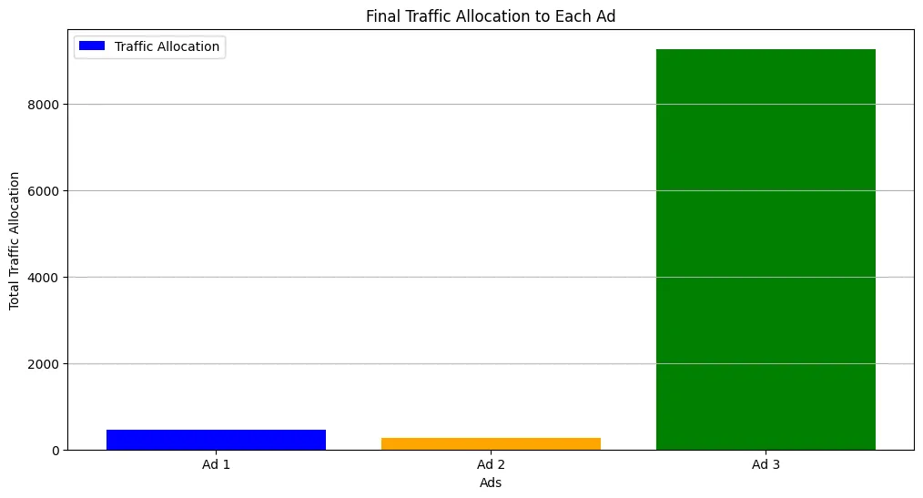
# Simulation three ads with different reward distributions
35
true_mean_rewards = [0.3, 0.5, 0.7]
36
reward_distributions = [lambda: np.random.binomial(1, p) for p in true_mean_rewards]
37

38
# Parameters
39
n_arms = len(true_mean_rewards)
40
c = 1
41
delta_min = min(true_mean_rewards)
42

43
# Initialize bandit
44
bandit = EpsilonGreedyBandit(n_arms, c, delta_min)
45

46
# Run simulation
47
n_rounds = 10000
48
rewards = []
49
ad_selections = []
50
cumulative_rewards = np.zeros(n_rounds)
51
traffic_allocation = np.zeros((n_rounds, n_arms))
52

53
for t in range(n_rounds):
54
    selected_ad = bandit.select_arm()
55
    ad_selections.append(selected_ad)
56
    reward = reward_distributions[selected_ad]()
57
    rewards.append(reward)
58
    bandit.update(selected_ad, reward)
59
    cumulative_rewards[t] = cumulative_rewards[t-1] + reward if t > 0 else reward
60
    traffic_allocation[t] = bandit.arm_counts
61

62
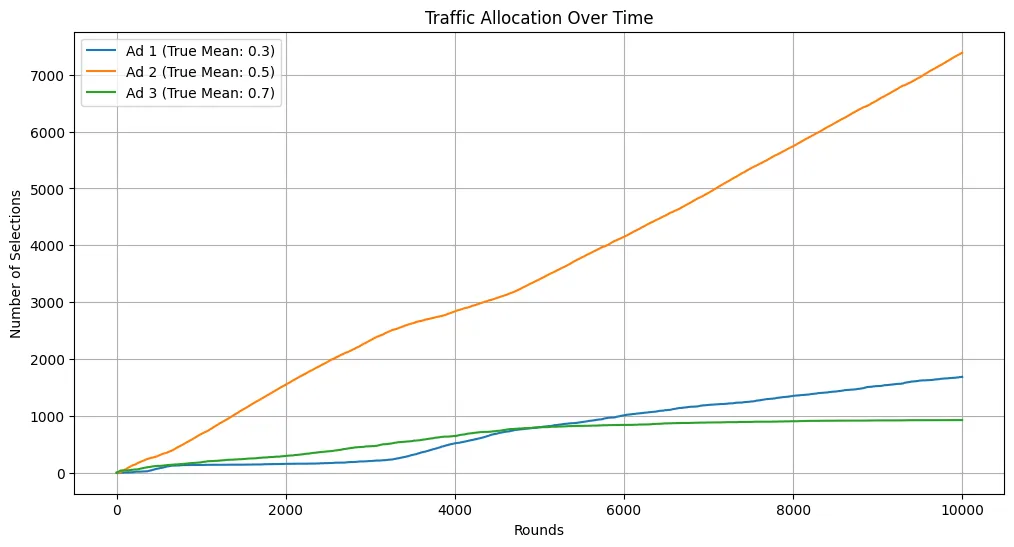
# Plot results
63
plt.figure(figsize=(12, 6))
64
for arm in range(bandit.n_arms):
65
    plt.plot(traffic_allocation[:, arm], label=f'Ad {arm+1} (True Mean: {true_mean_rewards[arm]})')
66
plt.title('Traffic Allocation Over Time')
67
plt.xlabel('Rounds')
68
plt.ylabel('Number of Selections')
69
plt.legend()
70
plt.grid()
71

72
# estimated
73
estimated_rewards = bandit.arm_rewards / (bandit.arm_counts + 1e-5)
74
plt.figure(figsize=(12,6))
75
plt.plot(range(n_rounds), cumulative_rewards, label='Cumulative Rewards', color='blue')
76
plt.xlabel('Rounds')
77
plt.ylabel('Total Reward')
78
plt.legend()
79
plt.grid()
80

81
# traffic allocation
82
plt.figure(figsize=(12,6))
83
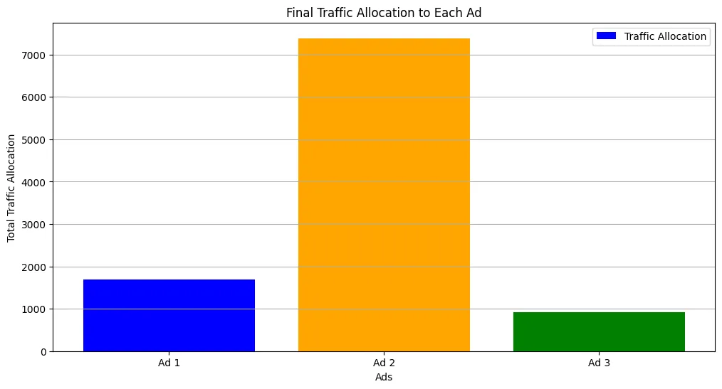
plt.bar(range(bandit.n_arms), traffic_allocation[-1], label='Traffic Allocation', color=['blue', 'orange', 'green'])
84
plt.xticks(range(bandit.n_arms), [f'Ad {i+1}' for i in range(bandit.n_arms)])
85
plt.title('Final Traffic Allocation to Each Ad')
86
plt.xlabel('Ads')
87
plt.ylabel('Total Traffic Allocation')
88
plt.legend()
89
plt.grid(True, axis='y')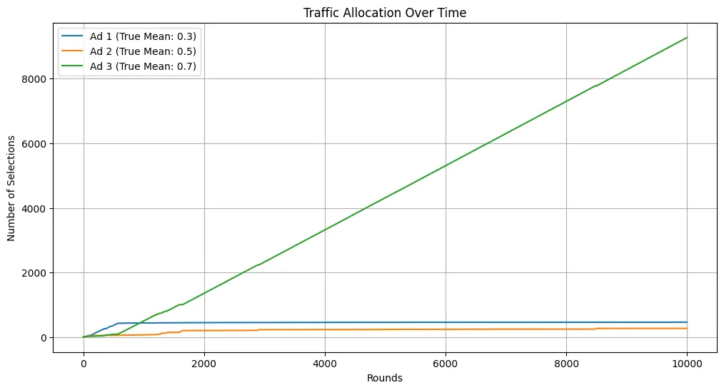

Traffic Allocation Over Time Cumulative Rewards Final Traffic Allocation to Each Ad

Example (Sampling Bandit Algorithm Implementation)

1
import numpy as np
2
import matplotlib.pyplot as plt
3

4
np.random.seed(42)
5

6
# Epsilon-Greedy Bandit Algorithm
7
class SamplingBandit:
8
    def __init__(self, n_arms):
9
        self.n_arms = n_arms
10
        self.alpha = np.ones(n_arms)
11
        self.beta = np.ones(n_arms)
12
        self.arm_rewards = np.zeros(n_arms) # cumulative rewards for each arm
13
        self.arm_counts = np.zeros(n_arms)  # number of times each arm was pulled
14
        self.total_counts = 0               # total number of pulls
15

16
    def select_arm(self):
17
        sample_means = np.random.beta(self.alpha, self.beta)
18
        return np.argmax(sample_means)
19

20
    def update(self, arm, reward):
21
        self.arm_rewards[arm] += reward
22
        self.arm_counts[arm] += 1
23
        self.total_counts += 1
24
        if reward == 1: # reward observed
25
            self.alpha[arm] += 1
26
        else: # no reward
27
            self.beta[arm] += 1
28

29
# Simulation three ads with different reward distributions
30
true_mean_rewards = [0.3, 0.5, 0.7]
31
reward_distributions = [lambda: np.random.binomial(1, p) for p in true_mean_rewards]
32

33
# Parameters
34
n_arms = len(true_mean_rewards)
35
c = 1
36
delta_min = min(true_mean_rewards)
37

38
# Initialize bandit
39
bandit = SamplingBandit(n_arms)
40

41
# Run simulation
42
n_rounds = 10000
43
rewards = []
44
ad_selections = []
45
cumulative_rewards = np.zeros(n_rounds)
46
traffic_allocation = np.zeros((n_rounds, n_arms))
47

48
for t in range(n_rounds):
49
    selected_ad = bandit.select_arm()
50
    ad_selections.append(selected_ad)
51
    reward = reward_distributions[selected_ad]()
52
    rewards.append(reward)
53
    bandit.update(selected_ad, reward)
54
    cumulative_rewards[t] = cumulative_rewards[t-1] + reward if t > 0 else reward
55
    traffic_allocation[t] = bandit.arm_counts
56

57
# Plot results
58
plt.figure(figsize=(12, 6))
59
for arm in range(bandit.n_arms):
60
    plt.plot(traffic_allocation[:, arm], label=f'Ad {arm+1} (True Mean: {true_mean_rewards[arm]})')
61
plt.title('Traffic Allocation Over Time')
62
plt.xlabel('Rounds')
63
plt.ylabel('Number of Selections')
64
plt.legend()
65
plt.grid()
66

67
# estimated
68
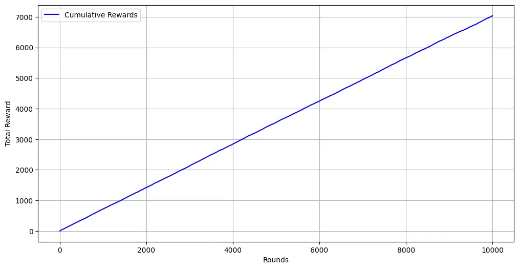
estimated_rewards = bandit.arm_rewards / (bandit.arm_counts + 1e-5)
69
plt.figure(figsize=(12,6))
70
plt.plot(range(n_rounds), cumulative_rewards, label='Cumulative Rewards', color='blue')
71
plt.xlabel('Rounds')
72
plt.ylabel('Total Reward')
73
plt.legend()
74
plt.grid()
75

76
# traffic allocation
77
plt.figure(figsize=(12,6))
78
plt.bar(range(bandit.n_arms), traffic_allocation[-1], label='Traffic Allocation', color=['blue', 'orange', 'green'])
79
plt.xticks(range(bandit.n_arms), [f'Ad {i+1}' for i in range(bandit.n_arms)])
80
plt.title('Final Traffic Allocation to Each Ad')
81
plt.xlabel('Ads')
82
plt.ylabel('Total Traffic Allocation')
83
plt.legend()
84
plt.grid(True, axis='y')

Traffic Allocation Over Time Cumulative Rewards Final Traffic Allocation to Each Ad