Problem Statement
-
Load data:
dt_simulated_weekly.csv -
Randomly select a hyperparameter set and do the adstock and saturation transformation
-
Fit the MMM model (single objective)
- Use the transformed variables.
- Assume a simple linear model,
-
Find the optimal budget allocation with an initial spend of $20,000 for each media.
Solution
Load Data
# import libraries and set seedimport pandas as pdimport numpy as npimport matplotlib.pyplot as pltfrom sklearn.linear_model import LinearRegressionfrom scipy.optimize import minimizenp.random.seed(42)- data 조작을 위해
pandas,numpy사용. - Task 에서 선형 모델을 가정하라고 하였기에
sklearn의LinearRegression을 사용. - 최적화 문제 해결을 위해
scipy.optimize의minimize사용. - 시각화를 위해
matplotlib.pyplot사용. - 재현성을 위해 시드 고정.
# load datadf = pd.read_csv('dt_simulated_weekly-1.csv')df.head()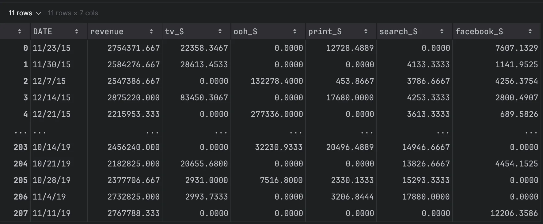
- 데이터는 주 단위로 수집된 시계열 데이터임을 확인할 수 있음.
- 각 컬럼의 의미는 다음과 같음:
DATE: 주 단위 시간 정보revenue: 매출 (종속 변수)tv_S,ooh_S,print_S,search_S,facebook_S: 광고 채널별 지출 (독립 변수)
결측치의 경우 없음을 확인하였으며, 실제 데이터에서는 결측치 처리 및 이상치 탐지 등의 전처리 과정이 필요할 수 있음.
Variable Transformation
# define media channelsmedia_channels = ['tv_S', 'ooh_S', 'print_S', 'search_S', 'facebook_S']
# define geometric adstock functiondef geometric_adstock(spend_series, decay_rate): adstocked_spend = np.zeros_like(spend_series, dtype=float) adstocked_spend[0] = spend_series[0] for i in range(1, len(spend_series)): adstocked_spend[i] = spend_series[i] + decay_rate * adstocked_spend[i-1] return adstocked_spend
# define hill saturation functiondef hill_saturation(adstocked_spend, alpha, gamma): epsilon = 1e-9 # prevent division by zero return 1 / (1 + ((gamma + epsilon)/adstocked_spend)**(alpha))
# set hyperparameters using random values within reasonable rangesdf_transformed = df.copy()hyperparameters = {}
for channel in media_channels: decay_rate = np.random.uniform(0.1, 0.9) alpha = np.random.uniform(1.0, 5.0) gamma = np.random.uniform(0.1, 1.0) * df[channel].mean()
# add hyper parameters for each channel hyperparameters[channel] = {'decay_rate': decay_rate, 'alpha': alpha, 'gamma': gamma}
# apply adstock / saturation transformations adstocked_spend = geometric_adstock(df[channel], decay_rate) saturated_spend = hill_saturation(adstocked_spend, alpha, gamma) df_transformed[f'{channel}_adstocked'] = adstocked_spend df_transformed[f'{channel}_saturated'] = saturated_spend
# check transformed data in dataframedf_transformed.head()- parent document 에서 언급한
geometric adstock transformation과hill saturation transformation을 각각 함수로 정의. - 각 광고 채널별로
decay rate,alpha,gamma의 hyperparameter 를 랜덤하게 설정하여 변환을 수행.- 각 변수의 범위 제한을 고려.
- saturation 의
gamma의 경우 채널별 평균 지출의 10% ~ 100% 사이로 설정.
- transformed variables 는 각각
_adstocked,_saturatedsuffix 를 붙여서 dataframe 에 추가.
Note (reference)
Randomly Selected Hyperparameters:
media channel: tv_S  - Adstock Decay Rate (theta): 0.3996  - Saturation Alpha (shape): 4.8029  - Saturation Gamma (scale): 11263.3120
media channel: ooh_S  - Adstock Decay Rate (theta): 0.5789  - Saturation Alpha (shape): 1.6241  - Saturation Gamma (scale): 10389.3799
media channel: print_S  - Adstock Decay Rate (theta): 0.1465  - Saturation Alpha (shape): 4.4647  - Saturation Gamma (scale): 2390.0664
media channel: search_S  - Adstock Decay Rate (theta): 0.6665  - Saturation Alpha (shape): 1.0823  - Saturation Gamma (scale): 5755.3140
media channel: facebook_S  - Adstock Decay Rate (theta): 0.7660  - Saturation Alpha (shape): 1.8494  - Saturation Gamma (scale): 565.6865
Saturation Curves:
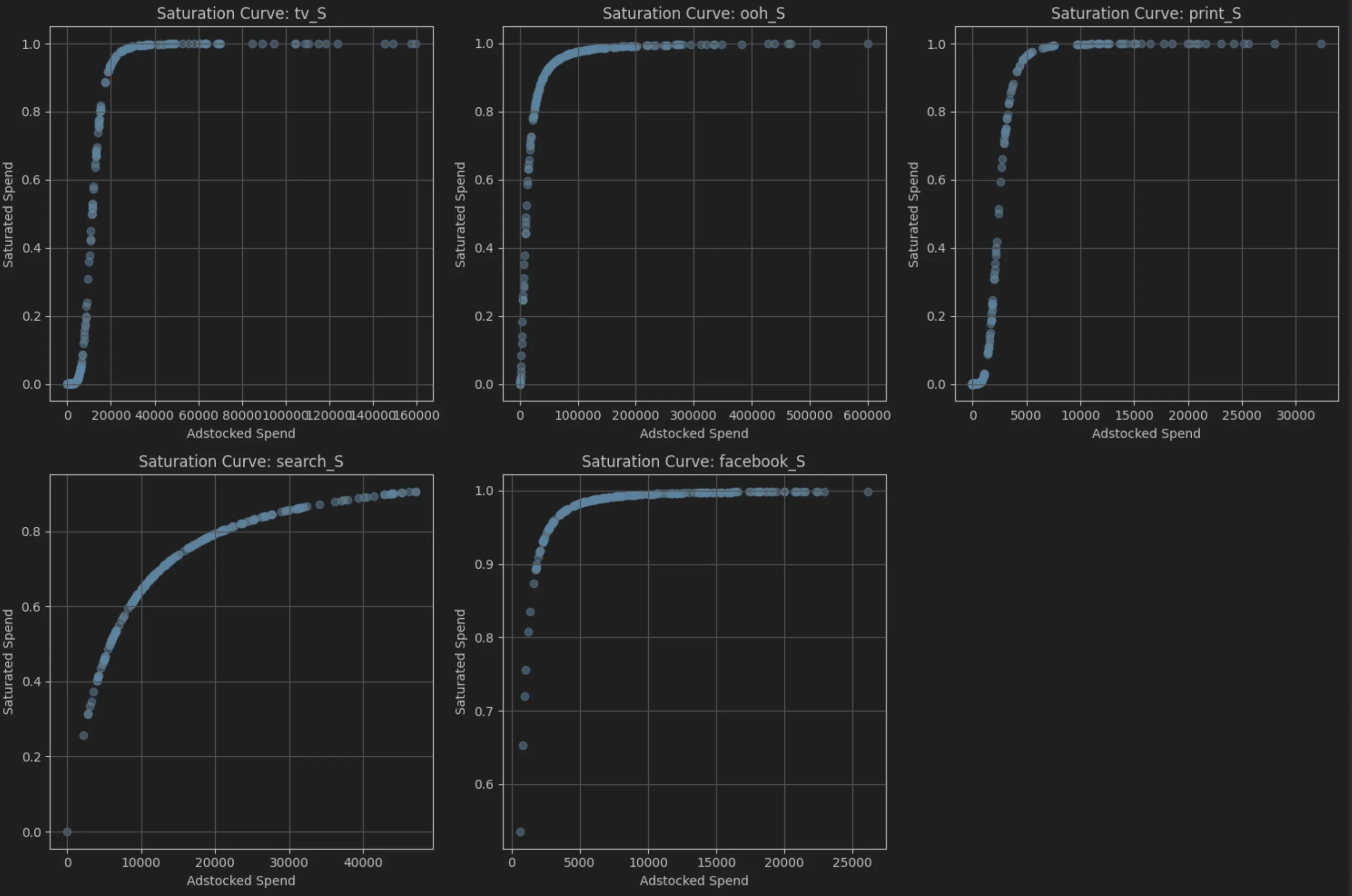
saturation 의 경우 “the law of diminishing returns” 를 반영하기에 adstock spend를 x축으로, saturated spend를 y축으로 하여 그리면 S-curve 형태가 됨을 시각적으로 확인할 수 있음.
Fit MdMM model using linear regression
# prepare X and yX = df_transformed[[f'{c}_saturated' for c in media_channels]]y = df_transformed['revenue']
# create and train linear regression modelmodel = LinearRegression()model.fit(X, y)r_squared = model.score(X, y)- Task 에서 제시한 선형 모델을 가정하여
saturated변수들로 독립변수 행렬X를 구성. - 종속변수
y는revenue로 설정. R-squared값을 통해 모델의 설명력을 평가 → 0.4927 (선형 모델로는 설명력이 다소 낮음을 확인할 수 있음)
Budget Allocation Optimization
budget allocation 의 경우 두 가지 접근법이 가능함:
- 과거 데이터의 바로 이후 기간에 대한 예산 할당을 최적화하는 접근 → 직전 데이터의
adstock_spend를 고려 필요. - adstock 효과를 무시하고 단순히 지출에 대한 saturation 효과만 고려하는 접근
1번 접근법:
# define revenue prediction functions for optimizationdef predict_revenue_with_consider_adstock_spend(spends, channels, h_params, intercept, coefs): transformed_spends = [] for i, channel in enumerate(channels): spend = spends[i] alpha = h_params[channel]['alpha'] gamma = h_params[channel]['gamma']
# use last date's adstocked spend * decay rate + current spend as adstocked spend # this assumes that we are right after the last date in the dataset and the adstock effect is still ongoing adstocked_spend = df_transformed[f'{channel}_adstocked'].iloc[-1] * h_params[channel]['decay_rate'] + spend saturated_spend = hill_saturation(adstocked_spend, alpha, gamma) transformed_spends.append(saturated_spend)
predicted_revenue = intercept + np.dot(transformed_spends, coefs)
# convert maximization problem to minimization return -predicted_revenue- 마지막 과거 데이터 (
208인덱스)의adstocked값을 고려하여 바로 다음 주의 지출을 최적화. adstocked값은 decay rate 를 곱하여 감소시킨 후, 현재 지출을 더하여 계산.saturated값은 앞서 정의한hill_saturation함수를 사용하여 계산.
최적화를 위해 maximization 문제를 minimization 문제로 변환.
2번 접근법:
def predict_revenue_ignore_last_adstock_spend(spends, channels, h_params, intercept, coefs): transformed_spends = [] for i, channel in enumerate(channels): spend = spends[i] alpha = h_params[channel]['alpha'] gamma = h_params[channel]['gamma']
# ignore last adstocked spend, just use current spend as adstocked spend # this assumes that the adstock effect has completely decayed by the time we are making the prediction saturated_spend = hill_saturation(spend, alpha, gamma) transformed_spends.append(saturated_spend)
predicted_revenue = intercept + np.dot(transformed_spends, coefs) return -predicted_revenueadstock효과를 무시하고 현재 지출만을 고려하여saturated값을 계산.- 이는 adstock 효과가 완전히 사라졌다고 가정하는 접근법.
Optimize Budget Allocation
1번 접근법:
# parameters for optimizationinitial_spends = [20000] * len(media_channels) # $20,000 per channeltotal_budget = sum(initial_spends) # $100,000constraints = ({'type': 'eq', 'fun': lambda spends: total_budget - np.sum(spends)}) # total budget constraintbounds = [(0, total_budget) for _ in media_channels] # non-negative spendsmodel_coefs = model.coef_ # get model coefficients
# perform optimizatonresult_consider_last_adstock_spend = minimize( fun=predict_revenue_with_consider_adstock_spend, x0=initial_spends, args=(media_channels, hyperparameters, model.intercept_, model_coefs), method='SLSQP', # bcs we have constraints bounds=bounds, constraints=constraints)
# print optimization results for both methodsif result_consider_last_adstock_spend.success: optimal_spends = result_consider_last_adstock_spend.x max_revenue = -result_consider_last_adstock_spend.fun
print("--- Budget Optimization Results considering Last Adstocked Spend ---") print(f"\nTotal Budget: ${total_budget:,.2f}")
allocation_df = pd.DataFrame({ 'Channel': media_channels, 'Optimal Spend': optimal_spends }) allocation_df['Percentage'] = (allocation_df['Optimal Spend'] / total_budget) * 100 print("\nOptimal Budget Allocation:") print(allocation_df.to_string(index=False, formatters={'Optimal Spend': '${:,.2f}'.format, 'Percentage': '{:.2f}%'.format}))
initial_predicted_revenue = -predict_revenue_with_consider_adstock_spend(initial_spends, media_channels, hyperparameters, model.intercept_, model_coefs)
print(f"\nExpected Maximum Revenue after Optimization: ${max_revenue:,.2f}") print(f"Expected Revenue with Equal Distribution: ${initial_predicted_revenue:,.2f}") print(f"Expected Revenue Uplift: ${max_revenue - initial_predicted_revenue:,.2f} ({(max_revenue/initial_predicted_revenue - 1)*100:.2f}%)")2번 접근법:
result_ignore_last_adstock_spend = minimize( fun=predict_revenue_ignore_last_adstock_spend, x0=initial_spends, args=(media_channels, hyperparameters, model.intercept_, model_coefs), method='SLSQP', # bcs we have constraints bounds=bounds, constraints=constraints)
if result_ignore_last_adstock_spend.success: optimal_spends_ignore = result_ignore_last_adstock_spend.x max_revenue_ignore = -result_ignore_last_adstock_spend.fun
print("\n--- Budget Optimization Results ignoring Last Adstocked Spend ---") print(f"\nTotal Budget: ${total_budget:,.2f}")
allocation_df_ignore = pd.DataFrame({ 'Channel': media_channels, 'Optimal Spend': optimal_spends_ignore }) allocation_df_ignore['Percentage'] = (allocation_df_ignore['Optimal Spend'] / total_budget) * 100 print("\nOptimal Budget Allocation:") print(allocation_df_ignore.to_string(index=False, formatters={'Optimal Spend': '${:,.2f}'.format, 'Percentage': '{:.2f}%'.format}))
initial_predicted_revenue_ignore = -predict_revenue_ignore_last_adstock_spend(initial_spends, media_channels, hyperparameters, model.intercept_, model_coefs)
print(f"\nExpected Maximum Revenue after Optimization: ${max_revenue_ignore:,.2f}") print(f"Expected Revenue with Equal Distribution: ${initial_predicted_revenue_ignore:,.2f}") print(f"Expected Revenue Uplift: ${max_revenue_ignore - initial_predicted_revenue_ignore:,.2f} ({(max_revenue_ignore/initial_predicted_revenue_ignore - 1)*100:.2f}%)")각 접근법의 결과는 다음과 같음:
--- Budget Optimization Results considering Last Adstocked Spend --- (1st approach)
Total Budget: $100,000.00
Optimal Budget Allocation:   Channel Optimal Spend Percentage      tv_S    $25,608.69     25.61%     ooh_S    $35,313.57     35.31%   print_S     $5,851.00      5.85%  search_S    $33,226.74     33.23%facebook_S         $0.00      0.00%
Expected Maximum Revenue after Optimization: $2,640,643.02Expected Revenue with Equal Distribution: $2,541,850.71Expected Revenue Uplift: $98,792.30 (3.89%)
--- Budget Optimization Results ignoring Last Adstocked Spend --- (2nd approach)
Total Budget: $100,000.00
Optimal Budget Allocation:   Channel Optimal Spend Percentage      tv_S    $23,459.44     23.46%     ooh_S    $27,002.46     27.00%   print_S     $5,118.77      5.12%  search_S    $36,701.82     36.70%facebook_S     $7,717.51      7.72%
Expected Maximum Revenue after Optimization: $2,527,572.87Expected Revenue with Equal Distribution: $2,362,181.37Expected Revenue Uplift: $165,391.49 (7.00%)- 두 접근법 모두 예산을 최적화하여 매출을 증가시킴을 확인할 수 있음.
- 1번 접근법의 경우가 adstock 효과과 고려되어 총 매출이 더 높게 나타남을 확인할 수 있음.